Introduction

AP Calculus AB is a rigorous course that requires students to have a strong understanding of the fundamental concepts of calculus. The formula sheet provided by the College Board is an essential tool for students to use during the exam. This sheet provides a comprehensive list of formulas that students need to know in order to succeed on the exam.
Sections of the Formula Sheet
The formula sheet is divided into the following sections:
- Limits and Continuity
- Derivatives
- Integrals
- Applications of Derivatives
- Applications of Integrals
Each section includes a list of formulas that are relevant to the corresponding topic.
How to Use the Formula Sheet
The formula sheet should be used as a reference during the exam. Students should familiarize themselves with the formulas on the sheet before the exam so that they can quickly find the formulas they need during the exam.
Important Tips
Here are some important tips for using the formula sheet:
- Know the formulas. Students should take the time to study the formulas on the sheet and make sure they understand how to use them.
- Use the sheet strategically. Students should not try to memorize all of the formulas on the sheet. Instead, they should focus on memorizing the most important formulas and then use the sheet to look up the formulas they need during the exam.
- Don’t waste time. Students should not spend too much time looking for a formula on the sheet. If they can’t find a formula quickly, they should move on and come back to it later.
Conclusion
The formula sheet is a valuable tool for students taking the AP Calculus AB exam. By following the tips above, students can use the sheet effectively to improve their score on the exam.
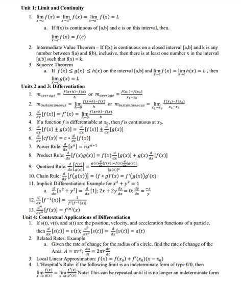
Section 1: Limits and Continuity
Limits
-
Definition of a Limit
> lim_(x->a) f(x) = L if for every ε > 0, there exists a δ > 0 such that if 0 < |x - a| < δ, then |f(x) - L| < ε. -
Properties of Limits
> * lim_(x->a) (f(x) + g(x)) = lim_(x->a) f(x) + lim_(x->a) g(x)
> * lim_(x->a) (f(x) – g(x)) = lim_(x->a) f(x) – lim_(x->a) g(x)
> * lim_(x->a) (cf(x)) = c lim_(x->a) f(x)
> * lim_(x->a) (f(x)g(x)) = lim_(x->a) f(x) lim_(x->a) g(x)
> * lim_(x->a) (f(x)/g(x)) = lim_(x->a) f(x)/lim_(x->a) g(x), if lim_(x->a) g(x) ≠ 0 -
L’Hôpital’s Rule
> If lim_(x->a) f(x) = lim_(x->a) g(x) = 0 or lim_(x->a) f(x) = lim_(x->a) g(x) = ±∞, then
> lim_(x->a) f(x)/g(x) = lim_(x->a) f'(x)/g'(x), if lim_(x->a) f'(x)/g'(x) exists.
Continuity
-
Definition of Continuity
> A function f(x) is continuous at a point a if
> * f(a) exists
> * lim_(x->a) f(x) = f(a) -
Properties of Continuous Functions
> * If f(x) and g(x) are continuous at a, then f(x) + g(x), f(x) – g(x), and cf(x) are continuous at a.
> * If f(x) and g(x) are continuous at a and g(a) ≠ 0, then f(x)/g(x) is continuous at a.
> * The composition of continuous functions is continuous.
Section 2: Derivatives
Definition of the Derivative
-
The derivative of a function f(x) with respect to x is defined as:
> f'(x) = lim_(h->0) (f(x + h) – f(x))/h
Properties of Derivatives
- The derivative of a constant function is 0.
-
The derivative of a power function is:
> f(x) = x^n, then f'(x) = nx^(n-1) - The derivative of a sum or difference of functions is the sum or difference of the derivatives.
-
The derivative of a product of functions is:
> f(x) = g(x)h(x), then f'(x) = g'(x)h(x) + g(x)h'(x) -
The derivative of a quotient of functions is:
> f(x) = g(x)/h(x), then f'(x) = (h(x)g'(x) – g(x)h'(x))/(h(x))^2 -
The chain rule:
> If f(x) = g(h(x)), then f'(x) = g'(h(x))h'(x)
Applications of Derivatives
- Finding the slope of a curve
- Finding the rate of change of a function
- Finding the maximum and minimum values of a function
- Finding the concavity of a function
- Finding the points of inflection of a function
Section 3: Integrals
Definition of the Integral
-
The integral of a function f(x) with respect to x is defined as:
> ∫f(x) dx = lim_(n->∞) Σ_(i=1)^n f(x_i*)Δx
Properties of Integrals
- The integral of a constant function is the product of the constant and the variable of integration.
- The integral of a sum or difference of functions is the sum or difference of the integrals.
- The integral of a product of a constant and a function is the product of the constant and the integral of the function.
- The integral of a quotient of functions is the quotient of the integrals.
-
The fundamental theorem of calculus:
> If f(x) is continuous on the interval [a, b], then ∫_a^b f(x) dx = F(b) – F(a), where F(x) is any antiderivative of f(x).
Applications of Integrals
- Finding the area under a curve
- Finding the volume of a solid
- Finding the work done by a force
- Finding the center of mass of a region
Section 4: Applications of Derivatives
Related Rates
- Related rates problems involve finding the rate of change of one variable with respect to another variable.
Optimization
- Optimization problems involve finding the maximum or minimum value of a function.
Curve Sketching
- Curve sketching involves graphing a function by using its derivative to find the critical points, intervals of increasing/decreasing, and concavity.
Section 5: Applications of Integrals
Area and Volume
- Area problems involve finding the area under a curve or between two curves.
- Volume problems involve finding the volume of a solid of revolution or a solid with known cross-sections.
Average Value
-
The average value of a function f(x) over an interval [a, b] is given by:
> (1/(b-a)) ∫_a^b f(x) dx
Work
-
The work done by a force F(x) over a distance d is given by:
> W = ∫_a^b F(x) dx
Center of Mass
-
The center of mass of a region R with density function ρ(x, y) is given by:
> (x̄, ȳ) = ((1/m) ∫∫_R xρ(x, y) dA, (1/m) ∫∫_R yρ(x, y) dA)
> where m is the mass of the region.