In AP Statistics, the binomial probability distribution is a fundamental concept used to determine the probability of a specific number of successes in a sequence of independent trials with a constant probability of success. The binomial CDF (cumulative distribution function) extends this concept by providing the cumulative probability of observing at least a specified number of successes.

Understanding the Binomial CDF
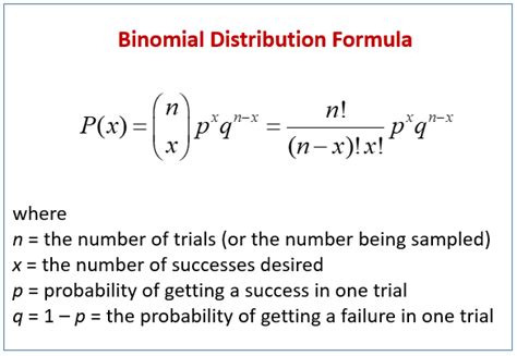
The binomial CDF, denoted as P(X ≥ k), represents the probability that a binomial random variable X takes on a value of k or greater. It is calculated as the sum of the probabilities of obtaining exactly k, k+1, k+2, …, n successes, where n is the total number of trials and p is the constant probability of success:
P(X ≥ k) = Σ P(X = i) for i = k to n
Applications of the Binomial CDF
The binomial CDF has numerous applications in various fields, including:
- Quality control: Determining the probability of a specified number or more defects in a manufactured product.
- Medical research: Assessing the efficacy of treatments by evaluating the probability of a certain number or more participants responding favorably.
- Voting predictions: Estimating the probability of a candidate receiving a minimum number of votes in an election.
- Financial modeling: Calculating the risk of portfolio losses exceeding a predetermined threshold.
Using the Binomial CDF Table
To simplify calculations, statisticians have developed a table of cumulative probabilities for the binomial distribution. This table provides P(X ≥ k) for various combinations of n, p, and k. By using the table, we can quickly determine the probability of at least a specified number of successes without having to perform tedious calculations.
Calculating the Binomial CDF in AP Statistics
In AP Statistics, students use statistical software or calculators to calculate the binomial CDF. Here’s an example using a calculator:
- Enter the values of n, p, and k into the appropriate function on your calculator.
- Press the “calc” key or equivalent to calculate the probability.
For instance, if n = 10, p = 0.4, and k = 4, the binomial CDF is P(X ≥ 4) = 0.6267.
Practical Examples
Example 1: Quality Inspection
A manufacturing plant produces widgets with a defect rate of 5%. A quality inspector randomly selects 20 widgets for inspection. What is the probability that at least 2 widgets are defective?
Solution:
n = 20, p = 0.05, k = 2
Using a binomial CDF table or calculator, we find that P(X ≥ 2) = 0.1129.
Example 2: Clinical Trial
A clinical trial evaluates the effectiveness of a new drug. It is hypothesized that at least 40% of participants will respond positively to the treatment. A sample of 50 participants is selected. What is the probability of obtaining a sample in which less than 40% respond positively?
Solution:
n = 50, p = 0.4, k = 19 (since 19 is the largest integer less than 40%)
Using a binomial CDF table or calculator, we find that P(X < 19) = 0.0065.
By understanding and applying the binomial CDF, students can accurately assess the probability of at least a given number of successes, enhancing their statistical analysis and decision-making abilities.