Introduction
The AP Calculus BC exam is a rigorous test that assesses students’ understanding of single-variable and multi-variable calculus. One of the essential elements of the exam is the equation sheet, which provides students with a list of essential formulas and identities. This sheet is a valuable resource that can help students save time and avoid errors during the exam.

**Section 1: Single-Variable Calculus**
Limits and Continuity
- Limit of a function: lim x->a f(x) = L
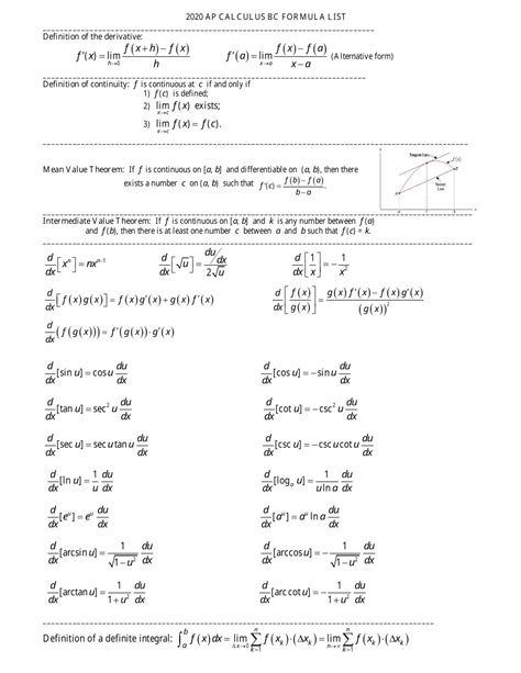
- Continuity: A function is continuous at x if
- f(a) is defined
- lim x->a f(x) = f(a)
Derivatives
- Derivative of a function: f'(x) = lim h->0 (f(x + h) – f(x))/h
- Power Rule: f(x) = x^n, then f'(x) = nx^(n-1)
- Product Rule: f(x) = g(x)h(x), then f'(x) = g'(x)h(x) + g(x)h'(x)
- Quotient Rule: f(x) = g(x)/h(x), then f'(x) = (h(x)g'(x) – g(x)h'(x))/h(x)^2
- Chain Rule: f(x) = g(h(x)), then f'(x) = g'(h(x)) * h'(x)
Integrals
- Indefinite Integral: ∫f(x) dx = F(x) + C
- Definite Integral: ∫a^b f(x) dx = F(b) – F(a)
- Fundamental Theorem of Calculus: If f(x) is continuous on [a, b], then ∫a^b f(x) dx = F(b) – F(a), where F(x) is an antiderivative of f(x).
Applications of Derivatives
- Critical points: Find f'(x) = 0 or f'(x) does not exist.
- Local maximums and minimums: If f'(x) = 0 and f”(x) < 0, then f(x) has a local maximum at x. If f'(x) = 0 and f''(x) > 0, then f(x) has a local minimum at x.
- Concavity: If f”(x) > 0, then f(x) is concave up. If f”(x) < 0, then f(x) is concave down.
- Related rates: Use derivatives to relate different rates of change.
Applications of Integrals
- Area: The area under the curve y = f(x) between x = a and x = b is given by ∫a^b f(x) dx.
- Volume: The volume of a solid generated by rotating the region under the curve y = f(x) between x = a and x = b about the x-axis is given by ∫a^b π[f(x)]^2 dx.
- Applications in physics: Integrals can be used to calculate displacement, velocity, and acceleration.
**Section 2: Multivariable Calculus**
Partial Derivatives
- Partial derivative with respect to x: f_x(x, y) = lim h->0 (f(x + h, y) – f(x, y))/h
- Partial derivative with respect to y: f_y(x, y) = lim h->0 (f(x, y + h) – f(x, y))/h
Multiple Integrals
- Double Integral: ∫∫R f(x, y) dA = lim Δx->0, Δy->0 ΣΣf(x_i, y_j)ΔxΔy
- Triple Integral: ∫∫∫R f(x, y, z) dV = lim Δx->0, Δy->0, Δz->0 ΣΣΣf(x_i, y_j, z_k)ΔxΔyΔz
Vector Calculus
- Dot product: a · b = |a||b|cosθ
- Cross product: a × b = |a||b|sinθ n
- Gradient: ∇f(x, y, z) = (f_x(x, y, z), f_y(x, y, z), f_z(x, y, z))
- Divergence: ∇ · F(x, y, z) = f_x(x, y, z) + f_y(x, y, z) + f_z(x, y, z)
- Curl: ∇ × F(x, y, z) = (f_z(x, y, z) – f_y(x, y, z)) i + (f_x(x, y, z) – f_z(x, y, z)) j + (f_y(x, y, z) – f_x(x, y, z)) k
**Section 3: Other Essential Formulas**
- Logarithmic identities: log_a(xy) = log_a(x) + log_a(y), log_a(x/y) = log_a(x) – log_a(y), log_a(a^x) = x
- Trigonometric identities: sin^2(x) + cos^2(x) = 1, tan(x) = sin(x)/cos(x), cot(x) = 1/tan(x)
- Geometric series: 1 + r + r^2 + … + r^n = (1 – r^(n+1))/(1 – r), |r| < 1
- Taylor series: f(x) = f(a) + f'(a)(x – a) + f”(a)(x – a)^2/2! + … + f^(n)(a)(x – a)^n/n!
**Tips and Tricks**
- Familiarize yourself with the equation sheet before the exam. Make sure you understand the formulas and can use them to solve problems.
- Use the equation sheet strategically. Don’t just memorize it; know when and how to apply the formulas.
- Don’t waste time re-deriving formulas. The equation sheet provides you with all the formulas you need.
- Check your answers. Use the equation sheet to verify your results and identify any errors.
**Common Mistakes to Avoid**
- Not checking your answers.
- Using the wrong formula.
- Making algebraic errors.
- Forgetting to apply the equation sheet strategically.
**Applications Beyond the Classroom**
The AP Calculus BC equation sheet has numerous applications beyond the classroom. It can be used to:
- Model real-world phenomena, such as the motion of objects, the flow of fluids, and the growth of bacteria.
- Design and optimize systems, such as bridges, aircraft, and medical devices.
- Analyze data and make predictions, such as in finance, marketing, and healthcare.