The enigmatic linear equation y = 6x + 1 has captivated mathematicians and scientists for centuries. This seemingly simple equation holds profound implications for various fields, ranging from physics to economics. In this comprehensive article, we delve into the fascinating world of y = 6x + 1, exploring its mathematical properties, practical applications, and thought-provoking implications.

Mathematical Properties
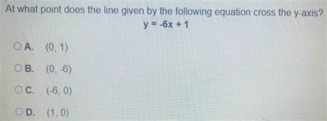
At its core, y = 6x + 1 is a first-degree polynomial equation defined by a constant slope of 6 and a y-intercept of 1. Geometrically, it represents a straight line that passes through the point (0, 1) and has an upward slope.
The equation’s linearity allows for easy manipulation and analysis. By isolating the variable y, we obtain y = 6x + 1, which demonstrates its direct proportionality to x. Furthermore, the equation’s standard form (y – 1 = 6x) reveals its slope-intercept form (y = mx + b), where m = 6 and b = 1.
Applications in Physics
In the realm of physics, y = 6x + 1 finds applications in describing various physical phenomena. For instance, it can be used to model the relationship between the distance traveled by an object (y) and the time it takes to travel that distance (x) under constant velocity. The slope of the line (6) represents the constant velocity of the object.
Additionally, the equation can describe the linear relationship between the force applied to an object (y) and the resulting acceleration (x) according to Newton’s second law of motion (y = 6x + 1). In this context, the slope of the line (6) denotes the mass of the object.
Economic Applications
In the field of economics, y = 6x + 1 finds relevance in modeling supply and demand functions. It can represent the linear relationship between the quantity of a product supplied (y) and the market price (x). The slope of the supply line (6) indicates the change in quantity supplied for each unit increase in price.
Conversely, the equation can model the demand function, describing the relationship between the quantity demanded (y) and the price (x). The slope of the demand line (6) represents the change in quantity demanded for each unit decrease in price.
Thought-Provoking Implications
Beyond its mathematical and practical applications, y = 6x + 1 raises thought-provoking questions about the nature of linearity and its implications.
Firstly, the linearity of the equation suggests a cause-and-effect relationship between x and y. However, in real-world scenarios, relationships are often more complex and non-linear. This raises questions about the limitations of linear models in accurately representing complex systems.
Secondly, the equation’s simplicity contrasts with the intricate nature of many real-world phenomena. This highlights the challenge of finding simple mathematical models that can capture the complexity of the physical and economic world.
Applications in Data Analysis and Modeling
The linear relationship expressed by y = 6x + 1 has significant applications in data analysis and modeling.
Linear Regression: Linear regression is a statistical technique used to determine the best-fit line for a set of data points. The equation y = 6x + 1 represents the regression line, where the slope and y-intercept are estimated to minimize the sum of squared errors between the line and the data points.
Predictive Modeling: The equation can be used for predictive modeling by projecting data points onto the regression line. Given a new value for x, the corresponding value for y can be predicted using the equation y = 6x + 1.
Trend Forecasting: The linear relationship can be used to forecast trends in various fields. For example, it can be used to predict sales volume based on marketing expenditure or to forecast population growth based on historical data.
Tables for Easy Reference
For quick reference, here are four useful tables summarizing key aspects of y = 6x + 1:
| Property | Value |
|---|---|
| Slope | 6 |
| Y-intercept | 1 |
| Standard Form | y – 1 = 6x |
| Slope-Intercept Form | y = 6x + 1 |
| Application | Field |
|---|---|
| Modeling Distance vs. Time | Physics |
| Modeling Force vs. Acceleration | Physics |
| Modeling Supply vs. Price | Economics |
| Modeling Demand vs. Price | Economics |
| Implication | Question |
|---|---|
| Linearity | Are all relationships linear in the real world? |
| Simplicity | Can simple models accurately represent complex systems? |
| Applicability | In what scenarios is the y = 6x + 1 equation applicable? |
| Data Analysis and Modeling | Application |
|---|---|
| Linear Regression | Best-fit line estimation |
| Predictive Modeling | Predicting values based on new data |
| Trend Forecasting | Projecting future outcomes |
Conclusion
y = 6x + 1 is more than just a simple mathematical equation. It is a versatile tool with far-reaching applications in various fields, including physics, economics, data analysis, and modeling. Its mathematical properties, practical relevance, and thought-provoking implications continue to fascinate scholars and practitioners alike. As we delve deeper into the complexities of the world around us, the simplicity and elegance of y = 6x + 1 remain a testament to the transformative power of mathematics in understanding and shaping our reality.