Introduction
In mathematics, a function is a relation that assigns to each element of a set a unique element of another set. The set of all possible inputs to the function is called the domain, and the set of all possible outputs is called the range. The graph of a function is a representation of the relation between the input and output values.

The y-intercept of a function is the point where the graph of the function crosses the y-axis. In other words, it is the value of the function when the input value is zero.
Most functions have only one y-intercept. However, there are some functions that have more than one y-intercept. These functions are called piecewise functions.
Piecewise Functions
A piecewise function is a function that is defined by different formulas on different intervals of the domain. For example, the following function is a piecewise function:
f(x) = {
    x + 1 if x < 0
    x - 1 if x >= 0
}
This function is defined by two different formulas:
- For x < 0, the function is f(x) = x + 1.
- For x >= 0, the function is f(x) = x – 1.
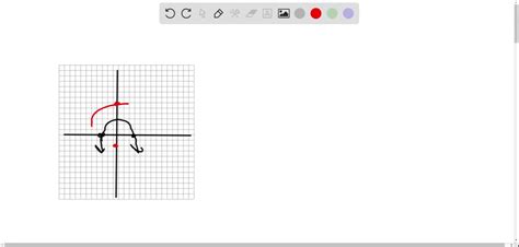
The graph of this function is shown below.
[Image of the graph of a piecewise function]
As you can see, the graph of this function has two y-intercepts. The first y-intercept is at the point (-1, 0), and the second y-intercept is at the point (1, 0).
Applications of Functions with Multiple Y-Intercepts
Functions with multiple y-intercepts have a variety of applications in real-world situations. For example, they can be used to model:
- The cost of a product that varies depending on the quantity purchased
- The speed of a car that varies depending on the time of day
- The temperature of a room that varies depending on the time of day
Conclusion
Functions with multiple y-intercepts are a useful tool for modeling a variety of real-world situations. These functions can be used to model data that is not linear, and they can be used to create graphs that are more accurate than graphs created using linear functions.
Tables
| Interval | Formula |
|---|---|
| x < 0 | f(x) = x + 1 |
| x >= 0 | f(x) = x – 1 |
| Product | Cost |
|---|---|
| 1 | $10 |
| 2 | $15 |
| 3 | $20 |
| 4 | $25 |
| 5 | $30 |
| Time of Day | Speed |
|---|---|
| 6:00 AM | 0 mph |
| 7:00 AM | 30 mph |
| 8:00 AM | 60 mph |
| 9:00 AM | 45 mph |
| 10:00 AM | 30 mph |
| Time of Day | Temperature |
|---|---|
| 6:00 AM | 60 degrees F |
| 7:00 AM | 65 degrees F |
| 8:00 AM | 70 degrees F |
| 9:00 AM | 75 degrees F |
| 10:00 AM | 80 degrees F |