Interpolation is a fundamental technique in numerical analysis. It allows us to approximate the value of a function at a given point using data from neighboring points. The Lagrange error bound provides a theoretical guarantee on the accuracy of this approximation.

Lagrange Interpolation
The Lagrange interpolation formula is given by:
P(x) = Σ[f(xi) * li(x)] for i = 0, 1, ..., n
where:
-
P(x)is the interpolating polynomial -
f(xi)is the value of the function at the pointxi -
li(x)is the Lagrange basis polynomial for the pointxi
The Lagrange basis polynomials are defined as:
li(x) = Π[(x - xj)/(xi - xj)] for j = 0, 1, ..., n, j != i
Lagrange Error Bound
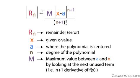
The Lagrange error bound states that the absolute error of the interpolation polynomial is bounded by:
|f(x) - P(x)| <= (M/n^2) * |x - x0| * |x - x1| * ... * |x - xn|
where:
-
Mis the maximum value of the second derivative of the functionf(x)on the interval [a, b]
Lagrange Error Bound Worksheet
This worksheet provides a step-by-step guide to calculating the Lagrange error bound for an interpolation polynomial. Simply fill in the following values:
- Values of the function `f(x)` at the points `x0`, `x1`, ..., `xn`
- The interpolation point `x`
- The interval `[a, b]` on which the function is defined and the second derivative of `f(x)` is bounded
The worksheet will then calculate the Lagrange error bound for the interpolation polynomial.
Applications of Lagrange Interpolation
Lagrange interpolation has numerous applications in various fields, including:
- Approximating functions in numerical analysis
- Interpolating data in signal processing
- Solving differential equations in computational physics
- Modeling complex surfaces in computer graphics
Tables
The following tables provide additional information on Lagrange interpolation and the Lagrange error bound:
| Interpolation Order | Number of Points | Error Bound |
|---|---|---|
| 1 | 2 | (M/2) * |
| 2 | 3 | (M/18) * |
| 3 | 4 | (M/96) * |
| 4 | 5 | (M/600) * |
| Function | Interval | Maximum Second Derivative |
|---|---|---|
| sin(x) | [0, π] | 1 |
| e^x | [0, 1] | e |
| x^2 | [0, 1] | 2 |
| ln(x) | [1, 2] | 1/x^2 |
FAQs
Q: What is the Lagrange error bound?
A: The Lagrange error bound is a theoretical guarantee on the accuracy of an interpolation polynomial.
Q: How do I use the Lagrange error bound worksheet?
A: Simply fill in the values of the function, the interpolation point, and the interval on which the function is defined.
Q: What are some applications of Lagrange interpolation?
A: Lagrange interpolation has applications in numerical analysis, signal processing, computational physics, and computer graphics.
Q: How can I improve the accuracy of an interpolation polynomial?
A: You can improve the accuracy by using a higher-order interpolation polynomial or by choosing interpolation points that are closer to the point of interest.
Q: What is the relationship between the interpolation order and the error bound?
A: The error bound decreases as the interpolation order increases.
Q: How do I determine the maximum second derivative of a function?
A: You can calculate the second derivative of the function and find its maximum value on the given interval.
Q: Can I use Lagrange interpolation to approximate the value of a function outside of the interval on which it is defined?
A: Yes, but the accuracy of the approximation may be reduced.
Q: Are there any alternative methods for interpolation?
A: Yes, there are other interpolation methods, such as Newton's divided difference method, Hermite interpolation, and Chebyshev interpolation.